Difference between revisions of "Temperature Scheduling in Simulated Annealing"
| Line 9: | Line 9: | ||
==ParSA Scheduling Capabilities== | ==ParSA Scheduling Capabilities== | ||
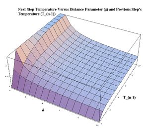
[[Image:Temp_delta.jpg|thumb|A rough portrayal of the dependence of the next temperature step as a function of the delta parameter and the previous temperature's value]] | [[Image:Temp_delta.jpg|thumb|A rough portrayal of the dependence of the next temperature step as a function of the delta parameter and the previous temperature's value]] | ||
| − | *SA_EasyScheduler | + | *'''SA_EasyScheduler''' |
-Warming Up | -Warming Up | ||
-Equilibrium | -Equilibrium | ||
-Cooling | -Cooling | ||
-Frozen | -Frozen | ||
| − | *SA_AartsScheduler | + | *'''SA_AartsScheduler''' |
-Warming Up | -Warming Up | ||
-Equilibrium | -Equilibrium | ||
-Cooling | -Cooling | ||
-Frozen | -Frozen | ||
| − | *SA_MIRScheduler | + | *'''SA_MIRScheduler''' |
-Warming Up | -Warming Up | ||
-Equilibrium | -Equilibrium | ||
Revision as of 19:36, 20 December 2007
<font; color="red"> THIS PAGE IS A WORK IN PROGRESS
The purpose of this page is to describe the notion of temperature scheduling in simulated annealing. The type of temperature schedule used in one's algorithm and the size and difficulty of terrain of the search space have connections to the convergence properties of ones algorithm. These topics are also considered briefly below, with an emphasis on the diamond problem. Additionally, prospective temperature scheduling strategies are also proposed, which will serve as a backbone to potential simulated annealing runs in the near future.
Introduction to Temperature Scheduling
<font; color="red"> Add description featured in D. Mitra et al about crystal growing annealing Temperature scheduling in simulated annealing refers to the process of controlling the temperature in a particular run through either geometric or adaptive means. The effect that temperature has on an annealing run is that it determines the probability that a solution with a higher cost function value will be accepted over one with a lower value, which is known as hill climbing. There are two main stages of temperature scheduling(warming up and cooling down), which are punctuated by two stopping conditions (equilibrium and frozen criterion respectively). The warming up stage represents a period during simulated annealing in which the temperature is raised to a high enough point that the probability of the acceptance of a neighboring solution is nearly one. Such a high probability of acceptance ensures that the final solution does not depend on the initial starting point. The warming period usually occurs for a predefined number of steps (known as a chain length). When the predefined number of steps have occurred, the annealing run has reached the equilibrium point, which simply is the term used to define the point at which warming has ended and cooling will begin. Continuing the analogy to classical annealing, the cooling stage of the annealing run, corresponds to the period during which the temperature is cooled down to reduce the acceptance ratio of lesser quality solutions. The cooling phase helps the algorithm to find an ultimate solution. Depending on the parameters set, the cooling phase is ended by either a set number of steps or a determined acceptance ratio lesser than some value. This point in the process is known as the freezing point (or frozen criterion).
ParSA Scheduling Capabilities
- SA_EasyScheduler
 -Warming Up
 -Equilibrium
 -Cooling
 -Frozen
- SA_AartsScheduler
 -Warming Up
 -Equilibrium
 -Cooling
 -Frozen
- SA_MIRScheduler
 -Warming Up
 -Equilibrium
 -Cooling
 -Frozen
Difficulty of the problem
The size and terrain of a particular search space are two concepts that one should include when speaking of the difficulty of a search space. The computing time drastically increases with the size (or dimensionality) of search space [1]. However, it is still possible to have higher dimensional problems that are unimodal or have very few local minima. Thus, one must also take into account the shape of search space when contemplating the difficulty.
In the diamond problem, a solution consists of values given to two amplitudes and three phases. The amplitudes represent the intensity of the light from the reference mirror and the diamond {the front and the back only differ by a constant). The phases represent each of the three surfaces: the reference mirror and the front and back of the diamond. Each of these quantities is represented by a certain order Legendre polynomial, which is represented in the form of a matrix with the number of rows and columns to match the order with an offset of one. Since the order Legendre Polynomial for each of the amplitudes and phases is set by the user, the dimensionality of the problem varies depending on the desired order. Thus, the lowest dimensionality that the diamond problem could take on would be 11 and the highest would be (cutting the Legendre polynomial order off at five) 125. However, it is most likely somewhere in between most likely slightly greater than 50, due to wanting to fully exploit the range of the Legendre polynomials to give the greatest accuracy in mapping the diamond surface.
Convergence and Simulated Annealing
- Markov Chains
- Random Walk
- Global Optimization
- ParSA-->[2]
Prospective strategies
References
[1] Esin Onbasoglu and Ozdamar, Yeditepe University, Istanbul, Turkey Journal of Global Optimization 2001
[2] Lee and Lee, Synchronous and Asynchronous Parallel Simulated Annealing with Multiple Markov Chains 1991
